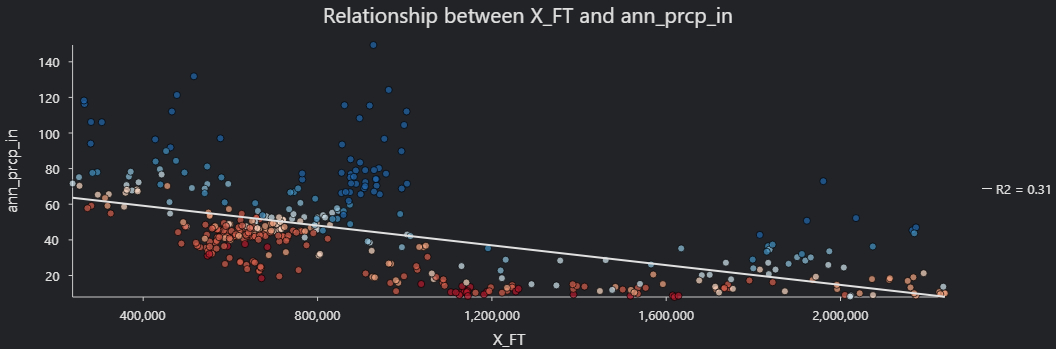
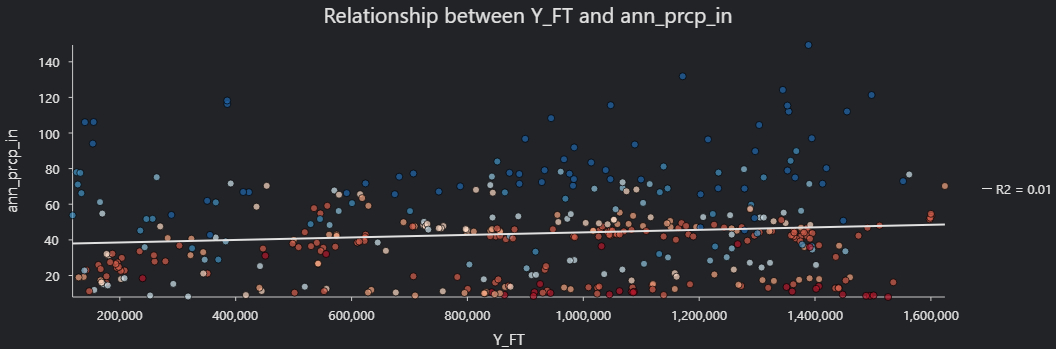
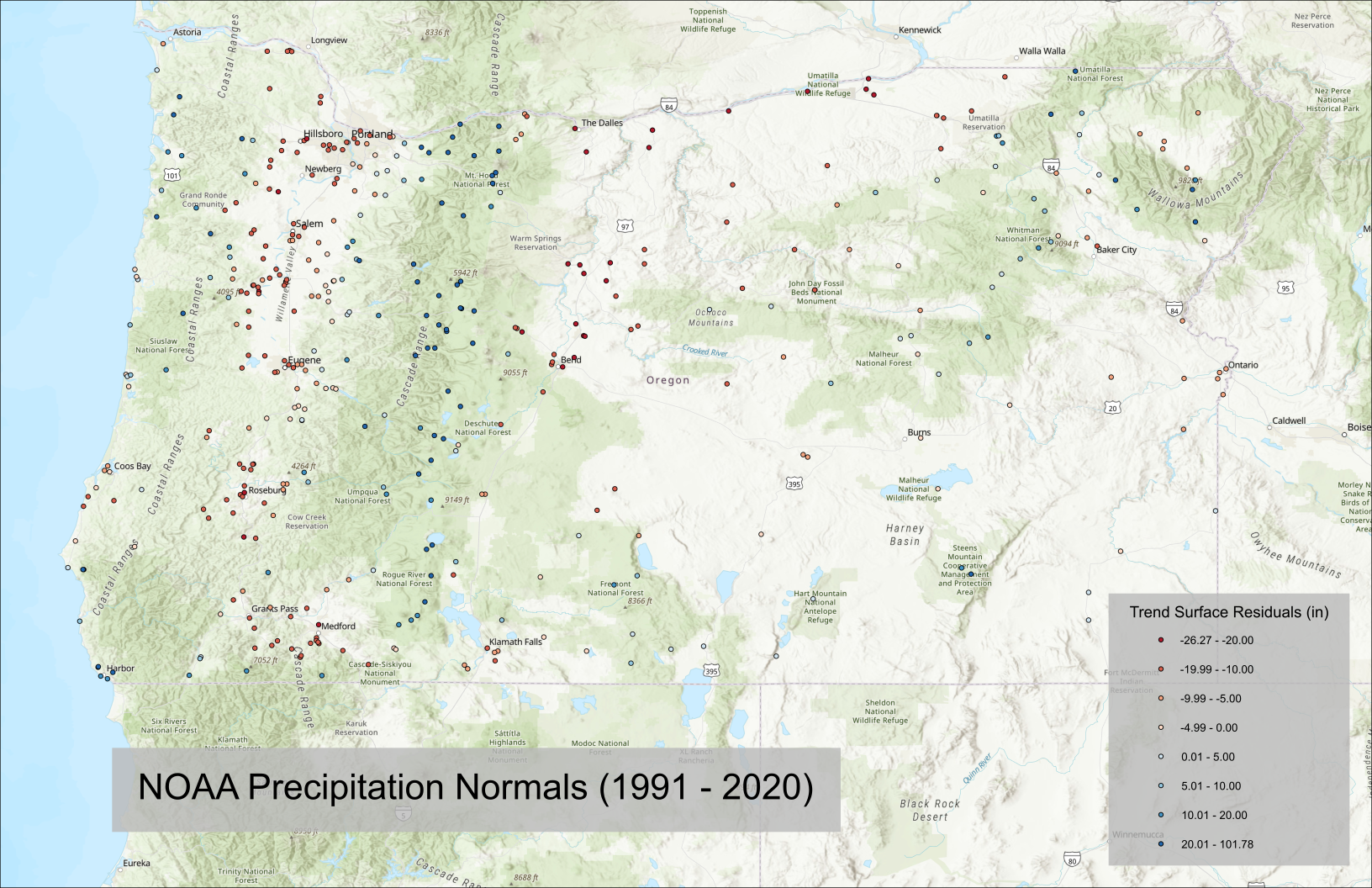
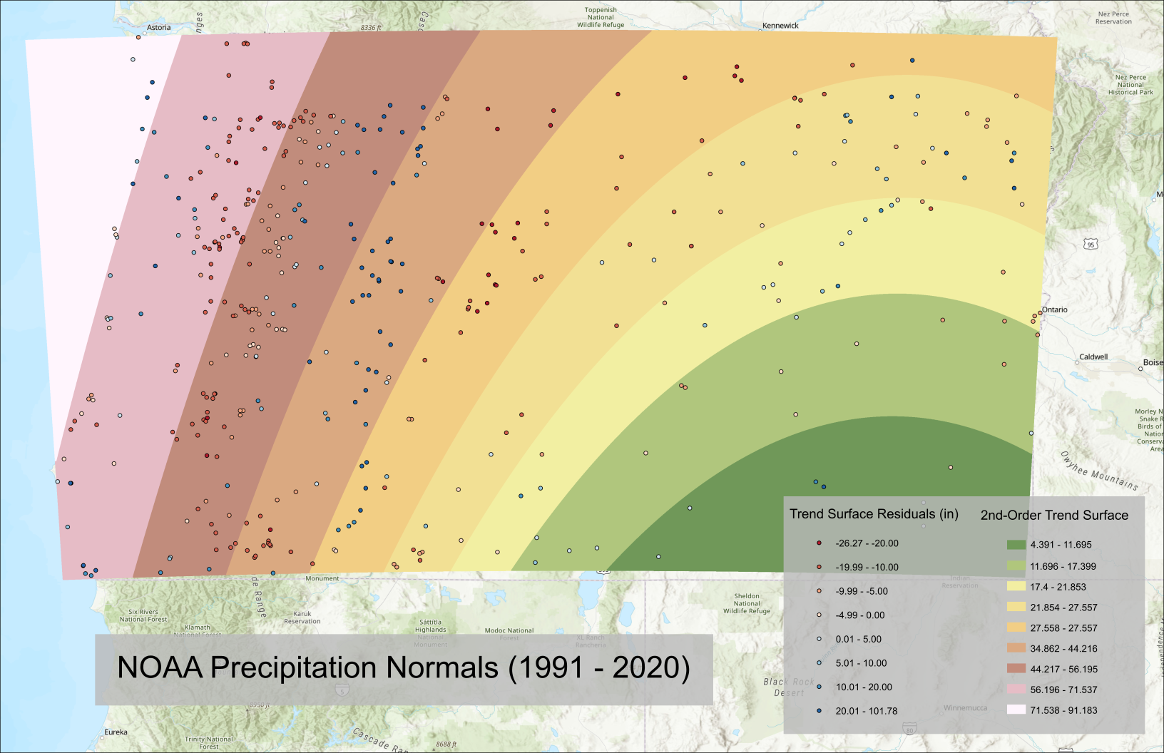
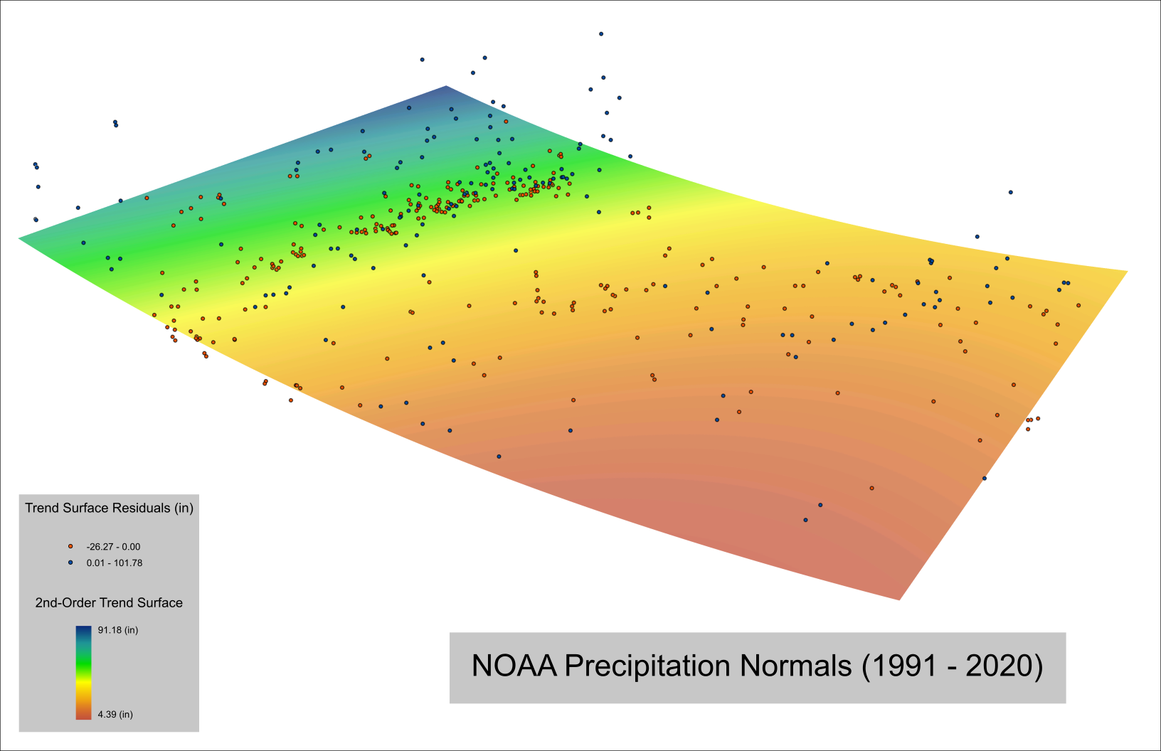
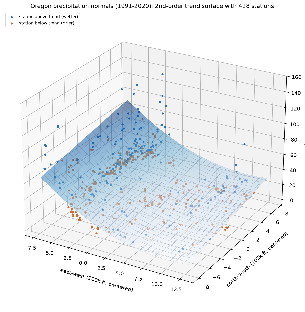
I fit polynomial trend surfaces (orders 1 through 5) to 428 NOAA precipitation
normals across Oregon, the same technique that produces a near-perfect regional
gradient for textbook examples like Kansas in Gimond's
Intro to GIS and Spatial Analysis. Oregon refused to cooperate:
R² plateaued around 0.41 even at higher
orders, and the zero-centered residual map redrew the Cascades and Coast Range out
of the leftover error. I ran Global Moran's I on the residuals to check whether that
visual clustering was real, and it was:
I ≈ 0.59, essentially unchanged from order 1
to order 3, since a low-order polynomial is nearly flat across any single station's
nearest neighbors and can't absorb mountain-range-scale structure. I built a 3D
scene in ArcGIS Pro (and a matching Python figure) with the fitted surface as a
floating sheet and each station suspended at its measured precipitation, so the
residual is a visible vertical gap. The finding: only about 40% of Oregon's rainfall
pattern is explained by location alone; the rest is exactly the local, spatially
autocorrelated structure that motivates kriging.
Global Moran's I, 428 stations (k = 8 nearest neighbors)
| Field |
Moran's I |
z-score |
| raw ann_prcp_in |
0.717 |
32.07 |
| residuals, order 1 |
0.594 |
26.64 |
| residuals, order 2 |
0.594 |
26.70 |
| residuals, order 3 |
0.594 |
26.66 |
All p < 0.000001. Removing the trend barely moves the ladder: the trend surface
operates at state scale, but Moran's I here is measuring neighbor-scale
clustering, so a bendier surface can't touch it. The autocorrelation lives at
mountain-range scale, not polynomial order.
Adapted from
Manuel Gimond's Intro to GIS and Spatial Analysis, ch. 12, run on Oregon data instead of the book's Kansas example.

 Selected work